The “dominant_eigenvalue” Tutorial

This short tutorial aims for an intuitive understanding of the functions and tools that are provided by the dominant_eigenvalue package. A complete code example to analyse the eigenvalues of the system is given for a simulated time series of the Ricker-type model with a fold bifurcation at around timestep \(t=9000\). In a second part an excercise with new datasets is prepared to improve the method handling and create more complicated plots.

Example 1: Eigenvalue analysis of a Ricker-type time series

First of all make sure that you import numpy and dominant_eigenvalue. In the code example numpy is abbreviated as “np”. Next you need to load the simulated Ricker-type time series that is already prepared in the``dominant_eigenvalue`` package. Make sure that you define the correct path of the dataset to avoid import errors of the dataset. The code could look like

import numpy as np
from antiCPy.early_warnings import dominant_eigenvalue
gendata_ricker_type=np.genfromtxt('ricker_type.csv', delimiter=',')
time_ricker_type = np.arange(gendata_ricker_type.size)

with a csv file. Now gendata_ricker_type is a numpy array with the time series data that we want to investigate. The sampling time array time_ricker_type is defined by sampling steps of unity due to the chosen simulation time step for the Ricker-type model. In order to estimate the dominant eigenvalues of the time delay embedded dynamical system with dominant_eigenvalue.analysis.AR_EV_calc we have to choose a suitable embedding dimension \(E\) and time delay \(\tau\). Several algorithms are available to optimize these parameters. First of all the embedding dimension is basically found by the dominant_eigenvalue.param_opt.false_NN function that is based on the false next neighbour algorithm. If a detailed analysis for various thresholds is desired the function dominant_eigenvalue.param_opt.various_R_threshold_fnn is the right choice. In this example we calculate an \(R_{\text{threshold}}\) series and plot the result via the dominant_eigenvalue.graphics.plot_fnn`` function. This can be implemented with

fnn_ricker_type = dominant_eigenvalue.param_opt.various_R_threshold_fnn(gendata_ricker_type,
                                                                        start_order = 1,
                                                                        end_order = 15,
                                                                        start_threshold = 15,
                                                                        end_threshold = 50)
dominant_eigenvalue.graphics.plot_fnn(fnn_ricker_type)

In the first step a numpy array fnn_ricker_type is created that contains in each row the number of false next neighbours from the dimensions 1 to 15 for a given threshold from 15 to 50. Each column contains the number of false next neighbours for one given dimensions over all thresholds in the predefined range. For the plot one has to adjust the extent in order to get reasonable axis labels. The offset 0.5 in the extent values fix the ticks in the center and are an esthetical artefact. If a quick analysis is convenient the false next neighbour algorithm can be applied just one time with dominant_eigenvalue.param_opt.false_NN. If you want to plot the results with dominant_eigenvalue.graphics.plot_fnn you need to set R_threshold_series = False` and the other parameters R_threshold and the dimension’s range start_order, end_order following your previous analysis. It could look like

fnn_ricker_type_II = dominant_eigenvalue.param_opt.false_NN(gendata_ricker_type)
dominant_eigenvalue.graphics.plot_fnn(fnn_ricker_type_II, R_threshold_series = False,
                                      R_threshold = '30', start_order = 1, end_order = 15)

It does not matter whether you apply a detailed or a quick analysis in that example. You will find that for an embedding dimension of \(d =3\) the number of false next neighbours tends to zero as shown in the figures cmap and quickfnn.

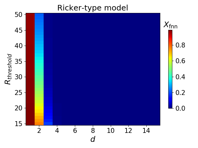
A color map of the \(R_{\text{threshold}}\) series.

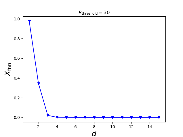
The fnn analysis for the specific \(R_{\text{threshold}} = 30\).

If a more complex analysis of the time delayed attractor is desired, a suitable time delay can be estimated via the average distance from diagonal algorithm that is provided by the dominant_eigenvalue.param_opt.avg_distance_from_diagonal function. The estimated distances can be visualized via the dominant_eigenvalue.graphics.plot_avg_DD function as shown in the following code and figure avg_DD:

tau_distances = dominant_eigenvalue.param_opt.avg_distance_from_diagonal(gendata_ricker_type, E = 3,
                                                                         start_lag = 1,
                                                                         end_lag = 10, image = False)
dominant_eigenvalue.graphics.plot_avg_DD(tau_distances)

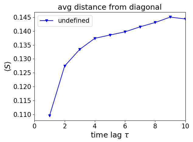
The average distance from diagonal results for the Ricker-type model.

The suitable time delay for an attractor reconstruction is often not crucial in order to derive the time development of the dominant eigenvalues with an autoregression scheme. The dominant_eigenvalue package provides with

A,B = dominant_eigenvalue.analysis.AR_EV_calc(gendata_ricker_type, 1200, 3)

dominant_eigenvalue.graphics.abs_max_eigval_plot(A, time_ricker_type, gendata_ricker_type, ws_1 = 1200,
                                                 axis = [0,10000,0.75,1.1], integrated_plot = True)

dominant_eigenvalue.graphics.max_eigval_gauss_plot(B, label_1 = 'Ricker-type model')

all necessary tools to

1. estimate the absolute values A of the dominant eigenvalue and all eigenvalues B in each rolling time window by using dominant_eigenvalue.analysis.AR_EV_calc,

2. plot the absolute dominant eigenvalue trend with or without plotting the investigated time series in the same window,

3. plot the dominant eigenvalues B in the complex Gaussian plane.

The chosen rolling time window length depends on the noise level of the data and is chosen as 1200 time sampling steps of the Ricker-type time series. The previously optimized embedding dimension of \(E=3\) is used. In the dominant_eigenvalue.graphics.abs_max_eigval_plot function it is necessary to give the same window size ws_1 as an input variable. Furthermore, it is possible to plot up to six eigenvalue time series and system variables at the same time and to choose a marker for the bifurcation point. In the dominant_eigenvalue.graphics.max_eigval_gauss_plot it is also allowed to plot up to three different sets of eigenvalues in the complex plane. For detailed information see The dominant_eigenvalue package documentation. The results for the Ricker-type model are shown in the figures DEV_ricker_type and gauss_ricker_type. The detrend option of dominant_eigenvalue.analysis.AR_EV_calc has been neglected in the tutorial to keep things simple. A proper nonlinear time series approach needs instead a suitable preparation via detrending if some deterministic slow trends are part of the data. With the detrending options described in The dominant_eigenvalue package documentation each window can be linearly detrended or a slow trend is estimated via a Gaussian filter and subtracted from the original non-stationary data.

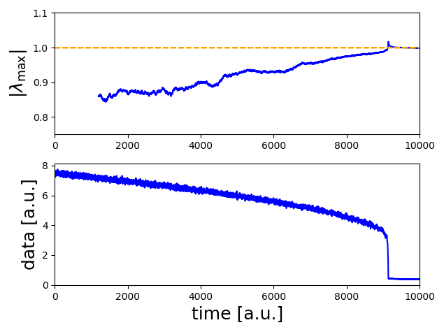
The absolute dominant eigenvalues’ trend with the Ricker-type time series.

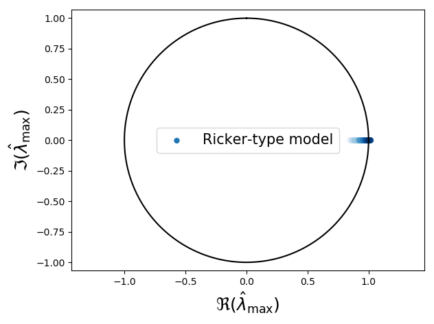
The dominant eigenvalues’ time evolution in the complex plane. Shading resolves the time from transparent to opaque.

If you make sure in the beginning to import the dominant_eigenvalue package as described above by `` from antiCPy.early_warnings import dominant_eigenvalue`` the whole example code can be run with the dominant_eigenvalue.tutorial.example() command that is pre-implemented in the dominant_eigenvalue package. The example will be processed without a time consuming threshold series or with dominant_eigenvalue.tutorial.example(threshold_series = True) with a threshold series. It can be alternatively copied out of that box

import numpy as np
from antiCPy.early_warnings import dominant_eigenvalue
# load the data
gendata_ricker_type=np.genfromtxt('ricker_type.csv', delimiter=',')
# create time sampling
time_ricker_type = np.arange(gendata_ricker_type.size)
# optimize embedding dimension with a time consuming, but detailed threshold series.
fnn_ricker_type = dominant_eigenvalue.param_opt.various_R_threshold_fnn(gendata_ricker_type,
                                                                        start_order = 1,
                                                                        end_order = 15,
                                                                        start_threshold = 15,
                                                                        end_threshold = 50)
dominant_eigenvalue.graphics.plot_fnn(fnn_ricker_type)
# otimize embedding dimension with a fast one threshold analysis
fnn_ricker_type_II = dominant_eigenvalue.param_opt.false_NN(gendata_ricker_type)
dominant_eigenvalue.graphics.plot_fnn(fnn_ricker_type_II, R_threshold_series = False,
                                      R_threshold = '30', start_order = 1, end_order = 15)
# otimize time delay
tau_distances = dominant_eigenvalue.param_opt.avg_distance_from_diagonal(gendata_ricker_type,
                                                                         E = 3, start_lag = 1,
                                                                         end_lag = 10,
                                                                         image = False)
dominant_eigenvalue.graphics.plot_avg_DD(tau_distances)
# estimate the absolute dominant eigenvalues and the eigenvalues per window
A,B = dominant_eigenvalue.analysis.AR_EV_calc(gendata_ricker_type, 1200, 3)
# plot the absolute dominant eigenvalue trend with the investigated dataset
dominant_eigenvalue.graphics.abs_max_eigval_plot(A, time_ricker_type, gendata_ricker_type,
                                                 ws_1 = 1200, axis = [0,10000,0.75,1.1],
                                                 integrated_plot = True)
# plot the dominant eigenvalues in the complex plane.
dominant_eigenvalue.graphics.max_eigval_gauss_plot(B, label_1 = 'Ricker-type model')

Example 2 (excercise): Analysis of two other simulated datasets

The package provides two additional simulated datasets: a time series of the Hénon model with a flip bifurcation and a time series of a map with a Hopf bifurcation. These additional time series and the Ricker-type model undergo a bifurcation around time \(t \approx 9000 [\text{a.u.}]\) and they can be loaded by

import numpy as np
from antiCPy.early_warnings import dominant_eigenvalue

ricker_type, henon, hopf = dominant_eigenvalue.tutorial.load_data()

In the end the results could look similar to these in the figures DEV_excercise and gauss_excercise.

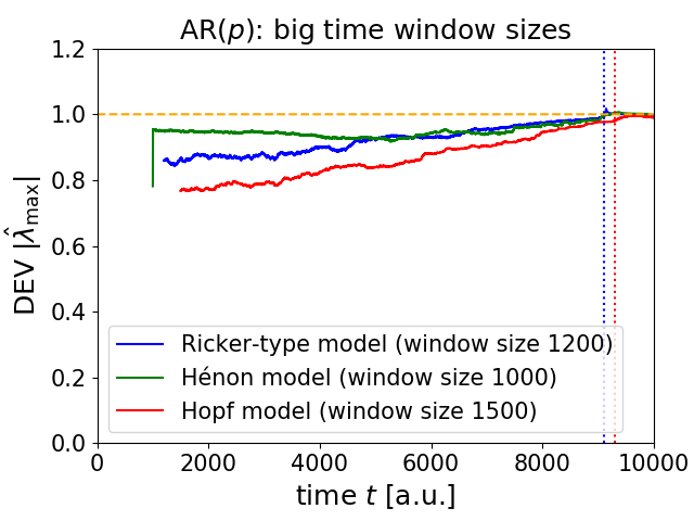
The total dominant eigenvalues’ trend of the three example models.

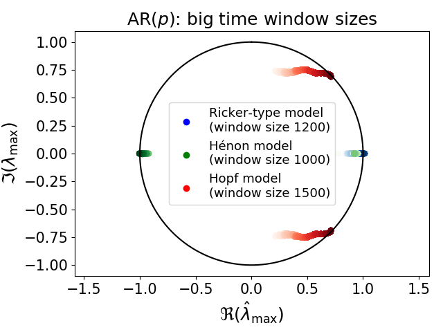
The dominant eigenvalues’ time evolution in the complex plane for the three example models. Shading resolves the time from transparent to opaque.